

ANALYSIS OF EXPERIMENTAL DATA
Our main concern when working in the lab is whether or not we have obtained the "right" answer. You should be aware, however, that it is not as straightforward as it might seem. Various research groups might have obtained different values for a physical constant. And although these values will differ from each other, they are all to be weighted equally in the absence of any other information. For that reason, accepted value is a better term. From now on we will take the comparison between our experimentally determined value and the accepted value as a measure of accuracy. When doing experiments, one must keep watch for two main types of error:
i. Random Errors; have a sign associated with them and that sign indicates whether the experimental value is high (+) or low (-) with respect to the accepted value. For example:
A musket ball is known to have a mass of 10.00 grams is weighted using a triple beam balance and the average of several trials is found to be 10.01 grams. The accuracy of the measurement is
This quantity is known as an absolute error, since the units of the error are the same as the units of the measurement. We might want to compute the relative error as well
Notice this quantity is unitless.
ii. Systematic Errors; these deviations can be divided into determinate and indeterminate errors. Determinate errors are errors which have a definite value that can, in principle, be measured and accounted for. Determinate errors, also called systematic errors, the most common sources are are instrumental, operator, and method errors.
Determinate errors are often unidirectional, that is they are all positive or all negative with respect to the accepted value. For example, another student weights the musket ball the next day using the same triple beam balance and the average of several trials is found to be 20.01 grams. The instrument is giving results which are too high. Let's take a look at the instrument...
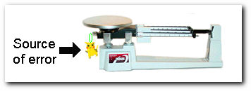
The failure of the experiment is the fault of a former operator. Someone who used the balance at an earlier time left a Pikachu key-chain hanged on the calibrating screw of the balance. This illustrates a combination of instrumental and operator error; the instrument's calibration is off but the current operator is responsible for checking that there are no foreign objects affecting the measurements.
Indeterminate Errors, also called random or statistical errors fluctuate randomly and do not have a definite value. For example, consider the titration data obtained by a student after doing five different measurements using a standard buret...

trial 1: 25.79 mL
trial 2: 25.77 mL
trial 3: 25.79 mL
trial 4: 25.77 mL
trial 5: 25.78 mL
The first three digits are the same in all cases; the last digit has an uncertainty associated with it. This uncertainty is the result of the buret's readability limit. Notice that the buret has ten subdivisions between each mL marking, so the buret can be accurately read to the nearest tenth of a mL and the next digit is uncertain. If we were to cut the last figure off; then the volume would be known only to the nearest tenth of a mL. If we keep that last digit, then the volume is known to the nearest hundredth of a mL; with some uncertainty indicative of the buret's readability limit.
Experimental data is made more meaningful by the inclusion of uncertainties. The value of the uncertainty gives one an idea of the precision inherent in a measurement of an experimental quantity. There are many ways to quantify uncertainty and the method used will depend upon how many measurements are made and on how crucial the reporting of the value of uncertainty is with regard to the interpretation of the experimental data.
REPORTING EXPERIMENTAL DATA
The students of the physical chemistry lab (this means you) are to report the value of a measured quantity x as the mean value
where xi is the ith measurement of x.
There will be an uncertainty associated with the reported value. The most widely used method for calculating uncertainty is representing it by the standard deviation of a series of measurements. This can be easily accomplished if it is assumed that a gaussian distribution function best describes the spread in the error values for a series of measurements made on a single observable.
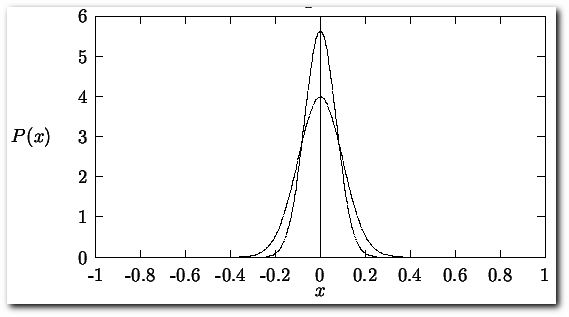
Here plotted for the case that μ = 0 and σ = 1 (broad peak) and μ = 0 and σ = 0.5 (narrow peak). The probability function P(x) is normalized,
implying that P(x) is a well-defined probability function. The average of x is given by
and that the point x = μ locates the peak of P(x) and, by symmetry, is also the mean.
The standard deviation σ can then be obtained from
Since P(x) represents the distribution of measured values about the mean μ, the result of any measurement has a ~66% chance of occurring in the range μ +/-sigma;
The second expression is known as the law of two sigmas.
The standard deviation is related to the width of the distribution of these errors. If σ has a small value, the probability function is narrow indicating that the probability of large errors is small. If σ has a large value, the probability function is broad indicating a high degree of probable errors. The above equations imply that σ can only be known exactly for a number of measurements N = ∞. Since the human life span is not long enough to make an infinite number of measurements, we must rely on estimates of the true σ, the best estimates of this parameter are given by the square root of the variance (S2 = the variance, S = square root of the variance)
Thus for multiple measurements N, the value that should be reported in the mean value and the uncertainty that should be reported is the 95% confidence level of the mean λ95 given by
where t is the student's t. For different numbers of independent measurements [N-1] the student's t has the following values...
| N-1 | 90% | 95% | 97.5% | 99.5% |
| 1 | 3.07766 | 6.31371 | 12.7062 | 63.656 |
| 2 | 1.88562 | 2.91999 | 4.30265 | 9.92482 |
| 3 | 1.63774 | 2.35336 | 3.18243 | 5.84089 |
| 4 | 1.53321 | 2.13185 | 2.77644 | 4.60393 |
| 5 | 1.47588 | 2.01505 | 2.57058 | 4.03212 |
| 10 | 1.37218 | 1.81246 | 2.22814 | 3.16922 |
| 30 | 1.31042 | 1.69726 | 2.04227 | 2.74999 |
| 100 | 1.29007 | 1.66023 | 1.98397 | 2.62589 |
| ∞ | 1.28156 | 1.64487 | 1.95999 | 2.57584 |
GRAPHICAL ANALYSIS - METHOD OF LIMITING SLOPES
The "method of limiting slopes" is the best technique for determining the uncertainty in the measurement of the slope and intercept of a linear plot. The following figure illustrates the method.
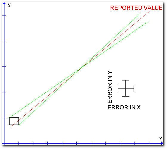
The technique consists of drawing a rectangle around every data point where the dimensions of the rectangle represent the uncertainties of the measured quantities. A best straight line is then drawn throughout the individual points. Two other lines which represent the maximum or minimum slopes are then drawn so that both lines pass through every rectangle. The differences in the slopes or intercepts of the limiting lines can be taken as twice the uncertainty in the slope or intercept of the best line.
PROPAGATION OF ERRORS
Suppose you are determining the density of a gold block, the density is a function of Mass and Volume
Each of the measured quantities has an error [+/-ΔM, +/-ΔL, +/-ΔH, +/-ΔW] associated with it. These errors will be carried through in some way to the error in the density +/-Δρ. For example, consider a small change in ρ from a small error in M
where ∂ρ/∂M is the partial differential of ρ with respect to M, the total error is obtained from
In general, the error λ for a quantity Ψ being calculated from the quantities x and y